

These days you can acquire time series data from multiple sources. In this article we will show you how to use InfluxDB, a popular time-series database dedicated to fast concurrent read/write of critical time-series information.
One can argue that using a traditional relational database may not work well with data in a time-series format because of the following:
- Every data source requires a custom schema. You need to spend more time deciding how to store your data, and if there are changes on the underlying data source then you may have to alter your table schema
- A traditional relational database doesn’t expire the data. You may only want to keep a certain window and then discard the rest automatically
- Time-series databases use an optimized storage format to make it fast for multiple clients to write and read the latest data, removing any worry about data duplicates, row lock contention, or other concurrent access issues.
InfluxDB offers integration with other time-series or data visualization tools out of the box (like Grafana, Python3) and it has a powerful yet simple language, called Flux, with which to run queries.
What you will require for this tutorial
- A docker or podman installation, so you can run InfluxDB. You can also do a bare metal installation, but we won’t cover that here and instead will use Podman. The InfluxDB documentation has very detailed installation instructions.
- InfluxDB 2.4.0 or better, We will use the Flux language on our queries, instead of FluxQL. NOTE: Flux will be dropped starting with InfluxDB 3.0. The OSS version will be called ‘InfluxDB Community‘.
- A linux distribution (e.g. Fedora Linux)
- Python3 and some experience writing scripts.
- Basic knowledge of relational databases, like MariaDB, can be useful, but is not required.
Running an InfluxDB server from a container
Using a container is probably the easiest way to get started.
We will use an external volume to persist the data across container reboots and upgrades (please check the container page to see all the possible options):
podman pull influxdb:latest
podman run --detach --volume /data/influxdb:/var/lib/influxdb --volume /data:/data:rw  --name influxdb_raspberrypi --restart always --publish 8086:8086 influxdb:latest
podman logs --follow influxdb_raspberrypi
Also, we are mapping an additional volume called /data directory inside the container, to import some CSV files later.
Next go to the machine where you are running InfluxDB (say http://localhost:8086) and complete the installation steps by:
- Creating a new user.
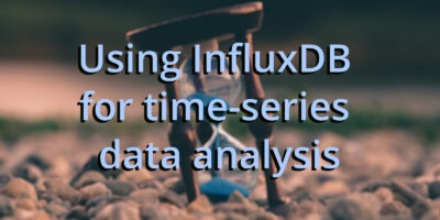
- Creating a bucket, with no expiration where we will put our data. Call it ‘COVID19’ (case sensitive).
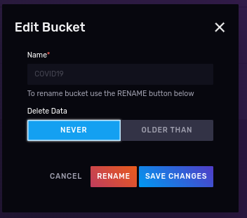
- Creating a read/write API token for that works only on the “COVID19” bucket
Working with data sets
In this tutorial we will use publicly available data from the Connection Data Portal.
COVID-19 in schools
The State of Connecticut provides numbers for the School COVID-19 cases through 2020-2022 in multiple formats, among other very useful information about the pandemic. For this tutorial, we will narrow our data exploration to 2 sets:
Importing data using an annotated CSV
We will use CSV data so it makes sense to get familiar how we can write it into the database the quickest and easiest way possible, allowing us to focus on analysis.
What do you want to learn from this dataset?
Ask questions about your data first before coding
In our case we want to see how many COVID cases happened over a period of time for a given school or city. Then you can decide to write queries, what data to discard, what to store, etc.
Let’s take a closer look at the data from these files:
| District | School ID | School name | City | School total | Report period | Date updated |
|---|---|---|---|---|---|---|
| XXXX School District | 1402 | XXXX YYYYYYYY School | XXXX | 0 | 10/08/2020 – 10/14/2020 | 06/23/2021 |
| XXXX School District | 1402 | XXXX YYYYYYYY School | XXXX | 0 | 10/15/2020 – 10/21/2020 | 06/23/2021 |
| XXXX School District | 1402 | XXXX YYYYYYYY School | XXXX | 0 | 10/22/2020 – 10/28/2020 | 06/23/2021 |
| XXXX School District | 1402 | XXXX YYYYYYYY School | XXXX | 0 | 10/29/2020 – 11/04/2020 | 06/23/2021 |
| XXXX School District | 1402 | XXXX YYYYYYYY School | XXXX | 0 | 11/05/2020 – 11/11/2020 | 06/23/2021 |
| XXXX School District | 1402 | XXXX YYYYYYYY School | XXXX | 0 | 11/12/2020 – 11/18/2020 | 06/23/2021 |
| XXXX School District | 1402 | XXXX YYYYYYYY School | XXXX | <6 | 11/19/2020 – 11/25/2020 | 06/23/2021 |
Normalizing your data will always be a priority regardless of which time-series database you use. Looking closer at the sample above we can see a few issues that show up in the very first lines:
- The report period: we could explode this measurement for the time period, but instead will select the first date of the selected range. This means we will see updates for each town, every 7 days.
- The school total: in some cases has indicators like <6. This is vague, so we will assume the upper limit (e.g 5).
- The school name: our interest is in the ‘School name’, ‘City’ and ‘Report period’. In the case of InfluxDB this constitutes a ‘data point’ and once defined it cannot be changed.
Then comes the decision on where and how to store the data. InfluxDB has the concept of tags and fields and measurements explained in understanding-Influxdb-basics:
- A bucket is nothing more than the database where the data will be stored. We will call ours ‘covid19’
- InfluxDB stores data into measurements (equivalent to a table in a relational database). Ours will be ‘schools’.
- Tags: are a combination of keys and values (e.g. city=xyz) and are used to annotate data. Each tag key and its corresponding value are treated as strings and do not change over time (think of them as metadata). In our case, the ‘School name’, ‘City’ are tags.
- Fields: the actual data being stored. Fields are typed and can be one of: int, float (default), or string. Though the values can change over time, their type is fixed and must be consistent over time. Any change to the field type would yield a new measurement and would complicate queries. In our example the ‘School total’ is a counter that will change with time.
- Time: the fabric of our data. Each datapoint requires a timestamp which can either be provided or can be auto-generated by InfluxDB. We will derive the timestamp from the ‘Report period’ and not from the date ‘updated fields’.
Annotating the CSV
InfluxDB needs help to figure out what is important for you, what needs to be indexed (to speed up search or group queries), what columns can be ignored, and where to put the data.
What does the CSV annotation look like? An example that describes our data should help:
District,School ID,School name,City,School total,Report period,Date updated
XXXX School District,1402,XXXX YYYYYYYY School,XXXX,<6,10/08/2020 - 10/14/2020,06/23/2021
If we break it down by column:
- Ignored columns: District, School ID, Date Updated. I will not skip the columns in the massaged file but rather tell the influx write to ignore them, as I want to show you how.
- Tags: School name, City
- Fields: School total,
- Timestamp: Report period. This needs to be expanded and also the date will be converted to RFC3339 (for example 1985-04-12T23:20:50.52Z). Dates also exploded for the period.
# datatype measurement,ignored,tag,tag,long,time,ignored
school,district,name,city,total,time,updated
"school","XXXX School District","XXXX YYYYYYYY School","XXXX",0,"2020-10-08T00:00:00Z","06/23/2021"
"school","XXXX School District","XXXX YYYYYYYY School","XXXX",0,"2020-10-15T00:00:00Z","06/23/2021"
"school","XXXX School District","XXXX YYYYYYYY School","XXXX",0,"2020-10-22T00:00:00Z","06/23/2021"
"school","XXXX School District","XXXX YYYYYYYY School","XXXX",0,"2020-10-29T00:00:00Z","06/23/2021"
...
We do also have 2 files so with a little help of a Python script we will massage the data:
#!/usr/bin/env python3
"""
This script massages CT COVID19 cases by school adding annotations for Influxdb, so they can be imported using the CLI.
"""
import csv
import datetime
import re
import sys
from argparse import ArgumentParser
from enum import Enum
from pathlib import Path

DEFAULT_REPORT = Path.home().joinpath("import_covid_data.csv")
MAX_ERRORS = 10

if __name__ == "__main__":
    PARSER = ArgumentParser("Convert CT school COVID19 data info an annotated CSV format for Influxdb")
    PARSER.add_argument('--destination', type=Path, default=DEFAULT_REPORT, help=f"Destination for massaged data. Default={DEFAULT_REPORT}")
    PARSER.add_argument('--explode', action='store_true',
                        help=f"Destination for massaged data. Default={DEFAULT_REPORT}")
    PARSER.add_argument('--max_errors', default=MAX_ERRORS, help=f"Maximum number of import errors, default {MAX_ERRORS}")
    PARSER.add_argument('source', nargs='+')
    ARGS = PARSER.parse_args()
    with open(ARGS.destination, 'w') as report:
        """
        Data normalization is a must; You can see than the format changed between 2020-2021 and 2021-2022:

        2020-2021: District,School ID,School name,City,School total,Report period,Date updated
        2021-2022: District,School Name,City,Report Period,Total Cases,Academic Year,Date Updated

        Also, order of total cases per school and report period flipped between years.

        To simplify things a little bit, we will drop a few columns from the resulting report
        2020-2021: School ID
        2021-2022: Academic Year

        Ending report will be:
        District,School Name,City,Total Cases,Report Period,Date Updated

        """
        report.write('''#datatype measurement,ignored,tag,tag,long,time,ignored
school,district,name,city,total,time,updated\n''')
        writer = csv.writer(report, delimiter=',', quotechar='"', quoting=csv.QUOTE_NONNUMERIC)
        num_errors = 0
        for data_file in ARGS.source:
            with open(data_file, 'r') as data:
                school_reader = csv.reader(data, delimiter=',')
                """
                Data format changed between year 2021-2022. Use the headers
                2020-2021: District,School ID,School name,City,School total,Report period,Date updated
                2021-2022: District,School Name,City,Report Period,Total Cases,Academic Year,Date Updated
                """
                original_format = True
                for row in school_reader:
                    try:
                        if row[0] == 'District':
                            original_format = row[1] == "School ID"
                            continue
                        if original_format:
                            class Position(Enum):
                                DISTRICT = 0
                                SCHOOL = 2
                                CITY = 3
                                TOTAL = 4
                                PERIOD = 5
                                UPDATED = 6
                        else:
                            class Position(Enum):
                                DISTRICT = 0
                                SCHOOL = 1
                                CITY = 2
                                TOTAL = 4
                                PERIOD = 3
                                UPDATED = 6
                        # Check for schools with less < 'cases' and take the upper limit (cases - 1)
                        matcher = re.search('<(\\d+)', row[Position.TOTAL.value])
                        if matcher:
                            total = int(matcher.group(1)) - 1
                        else:
                            total = int(row[Position.TOTAL.value])
                        date_ranges = row[Position.PERIOD.value].strip().split('-')
                        # Date in RFC3339
                        start = datetime.datetime.strptime(date_ranges[0].strip(), '%m/%d/%Y')
                        district = row[Position.DISTRICT.value]
                        school_name = row[Position.SCHOOL.value]
                        updated = row[Position.UPDATED.value]
                        city = row[Position.CITY.value]
                        if not ARGS.explode:
                            writer.writerow(
                                ["school", district, school_name, city, total, start.isoformat('T') + 'Z', updated])
                        else:
                            end = datetime.datetime.strptime(date_ranges[1].strip(), '%m/%d/%Y')
                            # We use a date generator
                            date_generated = (start + datetime.timedelta(days=x) for x in range(0, (end - start).days + 1))
                            for date in date_generated:
                                writer.writerow(["school", district, school_name, city, total, date.isoformat('T') + 'Z', updated])
                    except ValueError:
                        print(f"Problem parsing line: {row}, {data_file}", file=sys.stderr)
                        num_errors += 1
                        if num_errors > ARGS.max_errors:
                            print(f"Too many errors ({num_errors}), cannot continue!")
                            raise
Then run the normalizer script:
scripts/massage_school_covid_data.py --destination data/COVID-19_Cases_in_CT_Schools_Annotated.csv data/COVID-19_Cases_in_CT_Schools__By_School___2020-2021_School_Year.csv data/COVID-19_Cases_in_CT_Schools__By_School___2021-2022_School_Year.csv
Next we call the InfluxDB container with these arguments:
- Mount the directory where the annotated file is as a volume
- Tell influx to write the location of the InfluxDB server with –host flag
- Optional: Run with the dryrun flag, to verify that the parsing is correct
An example run with podman, on the machine where I have the data file, looks like the following (If you notice, I’m running on a disposable container, just to check the file syntax):
podman run --rm --tty --interactive --volume $HOME/Documents/InfluxDBIntro/data:/mnt:ro influxdb:latest influx write dryrun --org Kodegeek --format csv --bucket covid19 --file /mnt/COVID-19_Cases_in_CT_Schools_Annotated.csv odegeek school,city=XXXX,name=XXXX\ YYYYYYYY\ School total=0i 1602115200000000000 school,city=XXXX,name=XXXX\ YYYYYYYY\ School total=0i 1602720000000000000 school,city=XXXX,name=XXXX\ YYYYYYYY\ School total=0i 1603324800000000000 school,city=XXXX,name=XXXX\ YYYYYYYY\ School total=0i 1603929600000000000 ...
Now let’s do the real import, using the API token we created during the instance setup:
token='Z6OtfhBAaNuCp6YoML-I8nMkNO_RemnF_MdjFX68y2DoOVxZrtT2UfQkOCJkw_kuFYQYyluDc_nQAqQ1Y1Oetg==' podman exec --interactive --tty influxdb_raspberrypi influx write --org Kodegeek --format csv --bucket COVID19 --file /var/lib/influxdb2/COVID-19_Cases_in_CT_Schools_Annotated.csv --token $token
If the tool shows no messages you may assume there were no errors, though it is better to check by exploring the data to see if there were any issues.
Exploring the data using Flux query language
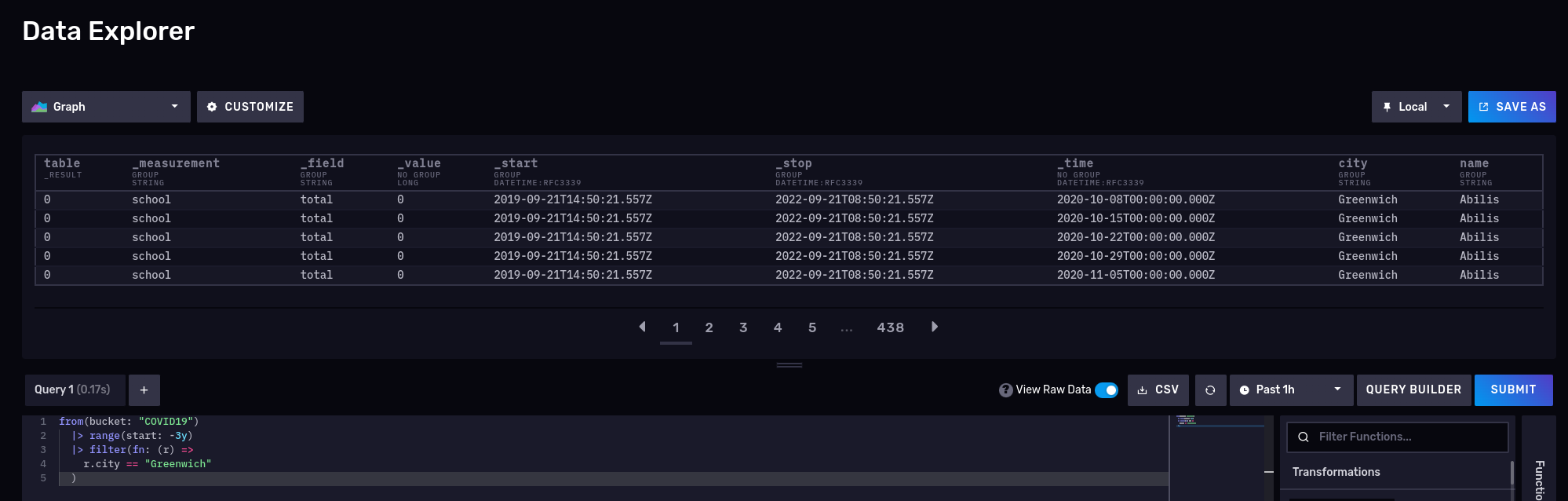
The easiest way to get a view of the raw data is with a small filter using the Flux language:
We know that we have a bucket called COVID19 (we can see all the buckets with the buckets() function), so we can try to list all measurements stored within the bucket by running the following commands (NOTE: the import statement is required):
import "influxdata/influxdb/schema"
schema.measurements(bucket: "COVID19")
This should return school, so no surprises here. Let’s try another one and query for the number of cases for the schools in Greenwich for the 2020-2022 period:
from(bucket: "COVID19")
  |> range(start: -3y)
  |> filter(fn: (r) => r.city == "Greenwich")
  |> yield()
What about a nice time series? Disable the raw mode and also switch to ‘Graph’:
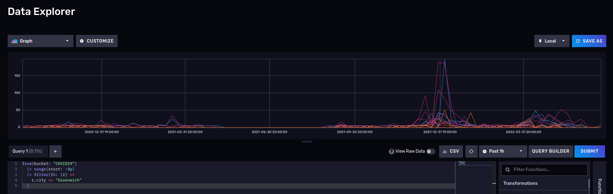
Please note that InfluxDB also supports Influxql, a SQL-like language from the 1.x releases, but some features in flux are not supported in influxql. influxql is skipped in this article.
TIP – To enlarge the images in this article:
It is necessary to view the images in a new tab or page to enlarge them.
More interesting queries
Number of COVID cases, by city
Cities with the highest number of cases
from(bucket: "COVID19")
    |> range(start: -3y)
    |> filter(fn: (r) => r._measurement == "school" and r._field == "total")
    |> group(columns: ["city"])
    |> drop(columns: ["name", "_start", "_stop"])
    |> sum()
And we can visualize it using a notebook:
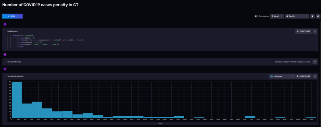
Most of the cities had around 200 cases, but keep in mind that these cities are small.
Flux is a functional language, and you can keep piping the results to other filters, transformations, or functions. Say, for sake of example, you now only want to see towns that had more than 7000 cases in the last 3 years:
from(bucket: "COVID19")
    |> range(start: -3y)
    |> filter(fn: (r) => r._measurement == "school" and r._field == "total")
    |> group(columns: ["city"])
    |> drop(columns: ["name", "_start", "_stop"])
    |> sum()
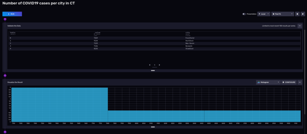
3 towns up to 7,800 cases, the rest left to Stamford with 8135 and Hartford with 9,134 cases.
Interesting things about this distribution:
- Single peak
- Right-skewed
- It looks like it is slightly Platykurtic
Let’s move on with a more complex dataset to see what else we can do with a time series and this tool.
Another dataset: Hartford Police Incidents from 01/01/2005 to 05/18/2021
But first, let’s learn about the city of Hartford:
Hartford is the capital and the fourth-largest city in Connecticut, an important industrial and commercial center of the country as well as the core city in the Greater Hartford metropolitan area, situated in the Connecticut River Valley. The city, located in the north-central part of the state, was settled on October 15, 1635, and named on February 21, 1637. It is a large financial center in the area and has become famous as the “insurance capital of the country”. It is considered to have a very strong economy, just like San Francisco and other leading economic hubs of the US. The city has also been home to several notable people such as famous authors Mark Twain and Harriet Beecher Stowe.
The Hartford police department collected information about crimes and made it publicly available on the Hartford data website:
In May 2021 the City of Hartford Police Department updated their Computer Aided Dispatch (CAD) system. This historic dataset reflects reported incidents of crime (with the exception of sexual assaults, which are excluded by statute) that occurred in the City of Hartford from January 1, 2005 to May 18, 2021
What is inside this dataset?
- 709K rows
- 12 columns:
| Description | Type | Column # |
|---|---|---|
| Case_Number | Number | 1 |
| Date | Date & Time | 2 |
| Time_24HR | Plain Text | 3 |
| Address | Plain Text | 4 |
| UCR_1_Category | Plain Text | 5 |
| UCR_1_Description | Plain Text | 6 |
| UCR_1_Code | Number | 7 |
| UCR_2_Category | Plain Text | 8 |
| UCR_2_Description | Plain Text | 9 |
| UCR_2_Code | Number | 10 |
| Neighborhood | Plain Text | 11 |
| geom | Location | 12 |
Grab a copy of the data for offline processing using curl:
curl --fail --location --output 'police-incidents-hartford-ct.csv' 'https://data.hartford.gov/api/views/889t-nwfu/rows.csv?accessType=DOWNLOAD&bom=true&format=true'
If we take a look at the data, we can see the following:
Case_Number,Date,Time_24HR,Address,UCR_1_Category,UCR_1_Description,UCR_1_Code,UCR_2_Category,UCR_2_Description,UCR_2_Code,Neighborhood,geom
21013791,05/10/2021,1641,123 XXX ST,32* - PROPERTY DAMAGE ACCIDENT,PROP DAM ACC,3221,,,0,CLAY-ARSENAL,"(41.780238042803745, -72.68497435174203)"
21014071,05/13/2021,0245,111 YYY ST,32* - PROPERTY DAMAGE ACCIDENT,PROP DAM ACC,3261,24* - MOTOR VEHICLE LAWS,EVADING RESP,2401,BEHIND THE ROCKS,"(41.74625648731947, -72.70484012171347)"
20036741,11/29/2020,1703,23456 ZZZ ST,31* - PERSONAL INJURY ACCIDENT,PERS INJ ACC,3124,23* - DRIVING LAWS,FOLL TOO CLOSE,2334,BEHIND THE ROCKS,"(41.74850755091766, -72.69411393999614)"
21013679,05/09/2021,2245,ZZZ AV & QQQQ ST,345* - PERSONAL INJURY ACCIDENT,PERS INJ ACC,3124,23* - DRIVING LAWS,TRAVELING TOO FAST,2327,UPPER ALBANY,"(41.778689832211015, -72.69776621329845)"
At first sight we can see it is not sorted, date and dates/times are in non-standard format, but otherwise it seems easy to normalize.
To complicate things a little more, the Uniform Crime Reporting (UCR)) codes have a separate document that explains their meaning.
ucr_code,primary_description,secondary_description
0100,homicide,homicide-crim
0101,homicide,murder-handgun
We will put all these measurements in different buckets with an expiration of never (normally your dataset points have an expiration date). For these 2 datasets we need to do some data manipulation so we will write a couple of importers using the Python SDK for maximum flexibility.
First import the Socrata UCR codes using a script (the following is a video image, enlarge to view):

And then import the police incidents using a different and slightly more complex script (police_case_importer.py) (The following is a video image, enlarge to view) :

The police_cases_importer.py also adds the ability to work with geolocation data inside InfluxDB. The code fragment that handles the insertion of a data point using the Python API write client is shown below…
Not so fast: What if the data is not sorted by time
from(bucket: "SocrateCodes") |> range(start: v.timeRangeStart, stop: v.timeRangeStop)
  |> filter(fn: (r) => r["_measurement"] == "socrata_ucr_codes")
  |> filter(fn: (r) => r._field == "ucr_code")
  |> group(columns: ["primary_description"])
  |> count(column: "_value")
  |> group(columns: ["_value", "primary_description"], mode: "except")
  |> sort(columns: ["_value"], desc: true)
  |> limit(n: 10)
The Hartford police department data is not strictly sorted by time but by case number which will definitely affect performance.
Queries can take a very long time to complete because the data is not properly sorted to begin with. This dataset is not terribly big (~ 112MB) so we make another change to the importer to sort the parsed collection in memory before inserting. This should provide some performance improvements during queries.
This sorting approach will not work for Gigabyte or Terabyte datasets so take care to use an external sorting mechanism, if required.
What we can learn from these police incidents public data
How many sub-types of crimes exist for each primary crime type code?
from(bucket: "SocrateCodes") |> range(start: v.timeRangeStart, stop: v.timeRangeStop)
  |> filter(fn: (r) => r["_measurement"] == "socrata_ucr_codes")
  |> filter(fn: (r) => r._field == "ucr_code")
  |> group(columns: ["primary_description"])
  |> count(column: "_value")
  |> group(columns: ["_value", "primary_description"], mode: "except")
  |> sort(columns: ["_value"], desc: true)
  |> limit(n: 10)
So we see the count per primary description. Also notice that we piped the output of the previous group query into another one, thus allowing us to fit the results into a single table:
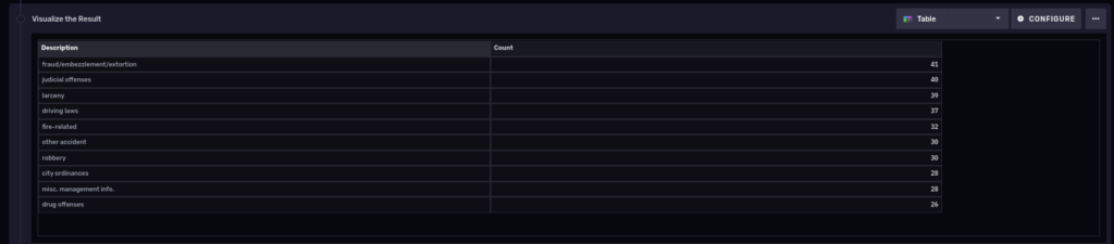
10 most common types of polices cases in the last 3 years
Let’s do something similar but to find out the 10 most common types of police cases in the last 3 years:
from(bucket: "PoliceCases")
    |> range(start: -3y)
    |> filter(fn: (r) => r._measurement == "policeincidents" and r._field == "ucr_1_code")
    |> group(columns: ["ucr_1_description"])
    |> drop(columns: ["neighborhood", "s2_cell_id", "lon", "lat", "ucr_2_category", "ucr_2_description", "ucr_2_code", "address"])
    |> count(column: "_value")
    |> group()
    |> sort(columns: ["_value"], desc: true)
    |> limit(n: 10)
NOTE: It turns out this query takes a long time to run on a tiny Raspberry PI 4 server for anything longer than 4 years. This is due to a known issue on the web interface that terminates your session too soon. If we write the query via the Python client instead we get:

Number of cases over time, grouped by week
We only need to truncate the precision of our ‘_time’ column to get a time series of the number of cases over time for a period of time. That will ‘group’ the results into buckets for us.
from(bucket: "PoliceCases")
    |> range(start: -3y)
    |> filter(fn: (r) => r._measurement == "policeincidents" and r._field == "case_number")
    |> truncateTimeColumn(unit: 1w)
    |> group(columns: ["case_number", "_time"])
    |> count()
    |> group()
And here is the result:
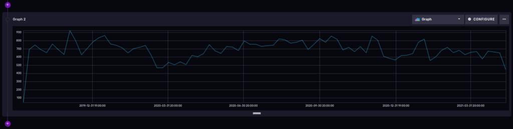
You could add the ucr_1_code number in the filter section of our flux query to be more specific about a certain type of crimes, but that is optional, of course.
Playing with geolocation data
At the time of this writing (influx 2.4.0) geolocation tagging is labeled as “experimental” on InfluxDB. Native support of geolocation capabilities inside the database is a very useful feature, let’s explore it next.
You could run the following on a notebook:
import "influxdata/influxdb/sample"
import "experimental/geo"
sampleGeoData = sample.data(set: "birdMigration")
sampleGeoData
    |> geo.filterRows(region: {lat: 30.04, lon: 31.23, radius: 200.0}, strict: true)
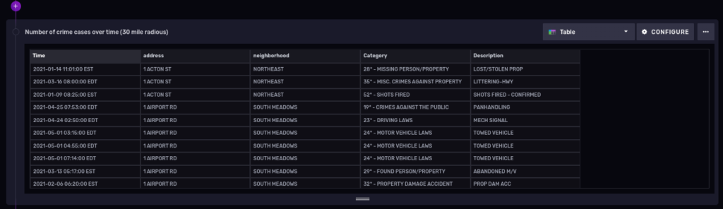
Coming back to our police cases dataset, can we find the number of crimes for the year 2021, within a radius of 30 miles of Hartford, CT?
First, a bit of geography:
Hartford, CT, USA Latitude and longitude coordinates are: 41.763710, -72.685097.
First let’s get a table with some data
from(bucket: "PoliceCases")
    |> range(start: 2021-01-01T00:00:00.000Z, stop: 2021-12-31T00:00:00.000Z)
    |> filter(fn: (r) => r._measurement == "policeincidents" and r._field == "lat" or r.field == "lon")
    |> group()
And now filter cases within a 30 mile (48.28032 Kilometer) radius from our Hartford coordinates:
import "experimental/geo"
from(bucket: "PoliceCases")
    |> range(start: 2021-01-01T00:00:00.000Z, stop: 2021-12-31T00:00:00.000Z)
    |> filter(fn: (r) => r._measurement == "policeincidents" and r._field == "lat" or r.field == "lon")
    |> geo.filterRows(region: {lat: 41.763710, lon: -72.685097, radius: 48.28032}, strict: false)
    |> group()
Let’s cover one more topic in detail before finishing.
Getting that data out of Influxdb using Python API
InfluxDB has a really nice feature that generates a code client from the UI. For our previous example, in Python:
from influxdb_client import InfluxDBClient

# You can generate a Token from the "Tokens Tab" in the UI
token = "<INFLUX_TOKEN>"
org = "Kodegeek"
bucket = "COVID19"

with InfluxDBClient(url="http://raspberrypi:8086", token=token, org=org) as client:
    query = """from(bucket: "COVID19")
    |> range(start: -3y)
    |> filter(fn: (r) => r._measurement == "school" and r._field == "total")
    |> group(columns: ["city"])
    |> drop(columns: ["name", "_start", "_stop"])
    |> sum()
    |> filter(fn: (r) => r._value >= 7000)
    |> sort(columns: ["_value"])"""
    tables = client.query_api().query(query, org=org)
    for table in tables:
        for record in table.records:
            print(record)
An example run may look like this (The following is a video image, enlarge to view):

FluxRecord() table: 0, {'result': '_result', 'table': 0, 'city': 'Fairfield', '_value': 7269}
FluxRecord() table: 1, {'result': '_result', 'table': 1, 'city': 'Hartford', '_value': 9134}
FluxRecord() table: 2, {'result': '_result', 'table': 2, 'city': 'New Haven', '_value': 7159}
FluxRecord() table: 3, {'result': '_result', 'table': 3, 'city': 'Norwalk', '_value': 7136}
FluxRecord() table: 4, {'result': '_result', 'table': 4, 'city': 'Stamford', '_value': 8135}
Other scripts can print a more polished version, but once you have access to the data you can do what you like!
Wrapping up
InfluxDB is one of the premiere dedicated time-series databases available in the opensource community. Influxdata, as a company, has taken great care to cultivate a collaborative and welcoming community for developers and users alike. This has resulted in a well-supported set of tools ready for Production use.
Some other items of interest include:
- The Connecticut OpenData portal has lots more interesting data sets you can download for free and learn about the state. I bet you have similar portals with public data where you live.
- If you write scripts in Python, you should definitely take a look at the examples from the Git repository.

That guy!
U+1F44D
Jose Nunez
Glad you like it!
Fred
A very interesting article.
Quite a bit above my knowledge level of DBs and programming but I hope to find time to explore it soon. Wow! CT provides much more information to the public than our state does…
Jose Nunez
They have a lot more of information there. If you are playing with data science or learning statistics this is a great place to get good datasets.
Renich Bon Ćirić
When attaching the volume using podman, you would require an SELinux label that allows writing. I would change the podman run command to:
“`
podman run –detach –volume ./influxdb:/var/lib/influxdb:Z –volume ./data:/data:Z –name influxdb_raspberrypi –restart always –publish 8086:8086 influxdb:latest
“`
In this case, the volumes will get mounted in a relative path from my current location. Also, I am using `:z` and `:Z` so that I use an SELinux label that allows for R and RW respectively.
I dunno about influxDBs internals but I deduced the first volume was to be read-only due to the original not having: `:rw` as a suffix.
Jose Nunez
That is correct, thanks a lot for the clarification.
Sean Maguire
According to https://www.influxdata.com/blog/the-plan-for-influxdb-3-0-open-source/ it would seem that the OSS version will not be called ‘InfluxDB Community’. The OSS version will be ‘InfluxDB Edge’, lacking features from the free-as-in-beer (and confusingly named) ‘InfluxDB Community’. The whole arrangement makes me wary of them.
Jose Nunez
It is early to say which direction they will take, I’m waiting to see the first releases of these packages to see how many changes were made to the original Influx distribution. In particular I liked the Flux language much more than the SQL like language they will support going forward, but at the end of the day is matter of resources and customer interest.
Markus
Hi,
first – thank you for this great Tutorial !
Just one Question – in sction
In this tutorial we will use publicly available data from the Connection Data Portal.
should the text to the Link not called: Connecticut Data Portal
instead of Connection Data Portal ?
Once again : thank’s for this great tutorial !